3 Quality checks

Code

# Import packages and working dataset
library(tidyverse)
library(haven)
library(plotly)
library(gt)

df_es <- readRDS("./data/ES2_NameSurvey_2025-09-09.RDS")

3.1 Repetition

Code

df_es |>
  mutate(
    Sex_DK = if_else(as.numeric(V001a) == 4, 1, 0),
    Region_DK = if_else(as.numeric(V001b) == 9, 1, 0),
    Religion_DK = if_else(as.numeric(V001e) == 7, 1, 0)) |>
  group_by(country_survey, id) |>
  summarise(across(ends_with("DK"), mean),.groups = 'drop') |>
  group_by(country_survey) |>
  summarise(across(ends_with("DK"), ~sum(.x == 1)), .groups = 'drop') |>
  gt() |>
  cols_label_with(fn =  ~str_remove(., "_DK"))

Table 3.1: Absolute number of respondents who answered “Don’t know” for all 10 names.

country_survey	Sex	Region	Religion
Belgium	5	14	55
Czech Republic	0	NA	29
Germany	1	10	42
Hungary	0	NA	20
Ireland	0	8	28
Spain	0	0	0
Switzerland	1	28	103
The Netherlands	6	20	58
UK	8	40	83

Code

df_es |>
  group_by(country_survey, id) |>
  summarise(across(c("V001a", "V001b", "V001e"), n_distinct),.groups = 'drop') |>
  group_by(country_survey) |>
  summarise(across(c("V001a", "V001b", "V001e"), ~sum(.x == 1)), .groups = 'drop') |>
  gt() |>
  cols_label(V001a = "Sex", V001b = "Region", V001e = "Religion")

Table 3.2: Absolute number of respondents who repeated the same answer for all 10 names.

country_survey	Sex	Region	Religion
Belgium	7	14	57
Czech Republic	1	640	89
Germany	6	10	45
Hungary	0	300	78
Ireland	9	9	32
Spain	0	0	0
Switzerland	19	30	110
The Netherlands	13	21	63
UK	18	42	87

3.2 Demographics

Here we check the difference in response pattern based on the respondent’s demographic variables. The table below show the average region congruence rates for Nigerian names.

Code

# Get weighted mean using the survey weight variable
get_mean <- function(var_es, wgt_es){
    weighted.mean({{var_es}}, w = {{wgt_es}}, na.rm = TRUE)
}

df_es <- 
  df_es |>
  mutate(resp_sex = case_match(VS1, 1 ~ "Male", 2 ~ "Female", .default = NA),
          #resp_edu = case_match(VS3, 1 ~ "No higher", 2 ~ "Higher", .default = NA),
          resp_age = case_when(VS2 < 25 ~ "18-24", VS2 > 24 & VS2 < 46 ~ "25-45", VS2 > 45 ~ "46+")) 

compare_cong <- function(country, group_comp){
  df_es |> 
    filter(country_name == country) |>
    group_by(country_survey, Name, group = get(group_comp)) |>
    summarise(region = get_mean(cong_region, Weging), .groups = 'drop') |>
    filter(!is.na(group)) |>
    group_by(country_survey, group) |>
    summarise(mean = mean(region), .groups = 'drop') |>
    pivot_wider(names_from = group, values_from = mean)
}
compare_cong("Nigeria", "resp_sex") |>
  left_join(compare_cong("Nigeria", "educ_adj")) |>
  left_join(compare_cong("Nigeria", "resp_age")) |>
gt() |> 
fmt_percent(decimals = 0) |>
sub_missing() |>
tab_spanner(label = "Sex", columns = c("Female", "Male")) |>
tab_spanner(label = "Education", columns = c("Lower than secondary", "Secondary +", "Other")) |>
tab_spanner(label = "Age group", columns = c("18-24", "25-45", "46+"))

Table 3.3: Average region congruence rate for Nigerian names by country and respondent’s characteristics.

country_survey	Sex		Education			Age group
country_survey	Female	Male	Lower than secondary	Secondary +	Other	18-24	25-45	46+
Belgium	14%	21%	17%	20%	10%	14%	18%	19%
Germany	31%	36%	33%	34%	16%	24%	33%	35%
Ireland	29%	37%	33%	34%	27%	28%	33%	34%
Spain	7%	17%	13%	11%	—	11%	9%	15%
Switzerland	32%	36%	32%	35%	28%	34%	36%	33%
The Netherlands	27%	31%	28%	30%	30%	21%	32%	30%
UK	34%	39%	34%	39%	34%	22%	35%	40%

3.3 Time

Important

The results below are based on the time spent in each session evaluating 10 names. Results refer to the second round only as the variable is not present in the first round data. The tables below also excludes sessions that took 60 minutes or more to be finalised (2.2%).

Code

df_es |> 
  filter(!is.na(Filltime_Total) & Filltime_Total < 3600) |>
  group_by(country_survey, region_es, input_1, Name) |>
  summarise(time_id = mean(Filltime_Total/60, na.rm = T), .groups = 'drop') |>
  group_by(country_survey) |>
  summarise(mean = mean(time_id), median = median(time_id),
            .groups = "drop") |>
  gt()  |>
  fmt_number(decimals = 1) |>
  opt_interactive(use_filters = TRUE, use_page_size_select = TRUE)

Table 3.4: Mean and median value of time (in minutes) spent in each session (evaluating 10 names)

Code

df_es |> 
  filter(!is.na(Filltime_Total) & Filltime_Total < 3600) |>
  ggplot(aes(x = Filltime_Total/60)) +
  geom_histogram(bins =  100) +
  facet_wrap(~country_survey) +
  theme_classic()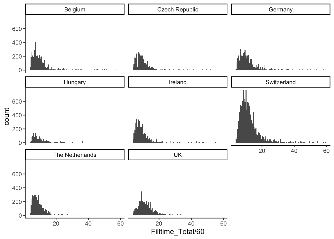

Figure 3.1: Distribution of time (in minutes) spent for 10 names in a session

Code

df_es |>
  filter(!is.na(Filltime_Total)) |>
  group_by(country_survey, id) |>
  summarise(time_id = mean(Filltime_Total/60), .groups = 'drop') |>
  group_by(country_survey) |>
  summarise(less_1min = sum(if_else(time_id < 1, 1, 0)),
            less_5min = sum(if_else(time_id < 5, 1, 0))) |>
  gt()

Table 3.5: Number of respondents who, on average, took less than 1 or less than 5 minutes to evaluate all ten names

country_survey	less_1min	less_5min
Belgium	0	30
Czech Republic	0	21
Germany	0	20
Hungary	0	10
Ireland	0	25
Switzerland	0	25
The Netherlands	0	32
UK	0	19